GeoJSON in R with the geojsonsf package

Have you ever wanted to convert between GeoJSON and sf objects in R, and do it quickly? Well now you can, with library(geojsonsf)

At Symbolix we do a lot of spatial analysis, and store our data in spatial databases - our favourite at the moment being mongodb, which stores (spatial) data as GeoJSON.

Therefore, I wanted a way to quickly convert between GeoJSON and sf. Hence this library.

geojsonsf has two main functions

• geojson_sf() - converts GeoJSON to sf objects
• sf_geojson() - converts sf objects to GeoJSON

GeoJSON to SF

Let's grab some GeoJSON of counties in the US

myurl <- "http://eric.clst.org/assets/wiki/uploads/Stuff/gz_2010_us_050_00_500k.json"
geo <- readLines(myurl)
geo <- paste0(geo, collapse = "")

To convert to an sf object, use geojson_sf

library(geojsonsf)
system.time({
  sf <- geojson_sf(geo)
})
#    user  system elapsed
#   0.215   0.022   0.238

That's right, less than a quarter of a second to convert 3,221 GeoJSON items into an sf object.

And because it's an sf object, you can use library(sf) to do with it what you will

library(sf) ## load sf to use their print methods
sf

# Simple feature collection with 3221 features and 6 fields
# geometry type:  GEOMETRY
# dimension:      XY
# bbox:           xmin: -179.1473 ymin: 17.88481 xmax: 179.7785 ymax: 71.35256
# epsg (SRID):    4326
# proj4string:    +proj=longlat +datum=WGS84 +no_defs
# First 10 features:
#    CENSUSAREA COUNTY         GEO_ID   LSAD      NAME STATE                       geometry
# 1     560.100    029 0500000US01029 County  Cleburne    01 POLYGON ((-85.38872 33.9130...
# 2     678.972    031 0500000US01031 County    Coffee    01 POLYGON ((-86.03044 31.6189...
# 3     650.926    037 0500000US01037 County     Coosa    01 POLYGON ((-86.00928 33.1016...
# 4    1030.456    039 0500000US01039 County Covington    01 POLYGON ((-86.34851 30.9943...
# 5     608.840    041 0500000US01041 County  Crenshaw    01 POLYGON ((-86.14699 31.6804...
# 6     561.150    045 0500000US01045 County      Dale    01 POLYGON ((-85.79043 31.3202...
# 7     777.093    049 0500000US01049 County    DeKalb    01 POLYGON ((-85.57593 34.8237...
# 8     945.080    053 0500000US01053 County  Escambia    01 POLYGON ((-87.16308 30.9990...
# 9     627.660    057 0500000US01057 County   Fayette    01 POLYGON ((-87.63593 33.8787...
# 10    574.408    061 0500000US01061 County    Geneva    01 POLYGON ((-85.77267 30.9946...

And of course we can plot it using my googleway package onto a Google Map.

library(googleway)

google_map() %>%
    add_polygons(sf[!gsf$STATE %in% c("02","15","72"), ], 
            fill_colour = "CENSUSAREA", 
            stroke_weight = 0)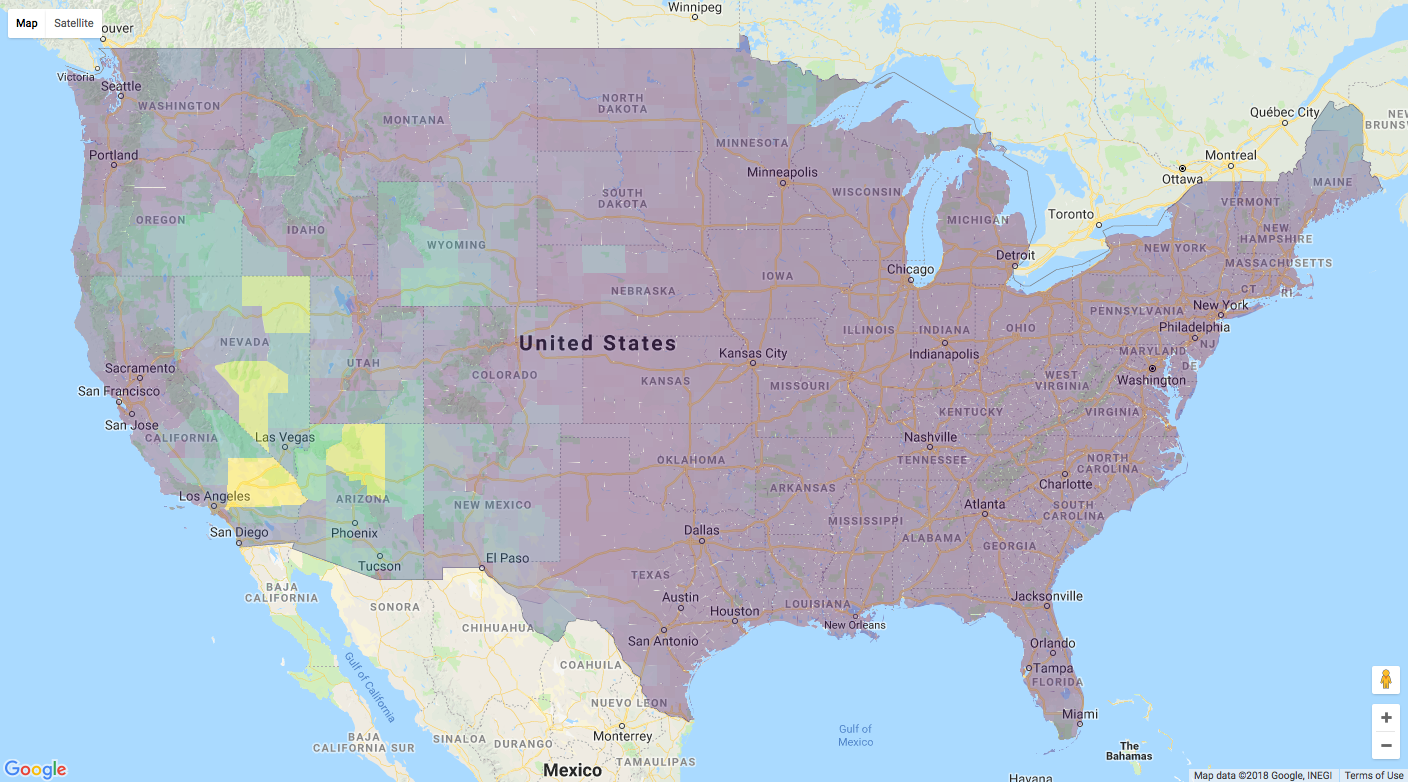

sf to GeoJson

Given our sf object we can now use sf_geojson() to covert back to GeoJSON

geo <- sf_geojson(nc)

str(geo)
# chr "{\"type\":\"FeatureCollection\",\"features\":[{\"type\":\"Feature\",\"properties\":{\"AREA\":0.114,\"PERIMETER\"| __truncated__

This gives you a string of GeoJSON.

If you want a separate object (i.e., a vector of GeoJSON) for each geometry, use atomise = TRUE

geo <- sf_geojson(nc, atomise = T)
str(geo)
# chr [1:100] "{\"type\":\"Feature\",\"properties\":{\"AREA\":0.114,\"PERIMETER\":1.442,\"CNTY_\":1825,\"CNTY_ID\":1825,\"NAME"| __truncated__ ...

This gives a vector of 100 features. This would be useful for storing each geometry in a spatial database, for example.